Training a Machine Learning Model- Container

This tutorial contains a Python application for training a deep learning model on EuroSAT dataset for tile-based classification task, and employs MLflow for monitoring the ML model development cycle. MLflow is a crucial tool that ensures effective log tracking and preserves key information, including specific code versions, datasets used, and model hyperparameters. By logging this information, the reproducibility of the work drastically increases, enabling users to revisit and replicate past experiments accurately. Moreover, quality metrics such as classification accuracy, loss function fluctuations, and inference time are also tracked, enabling easy comparison between different models.

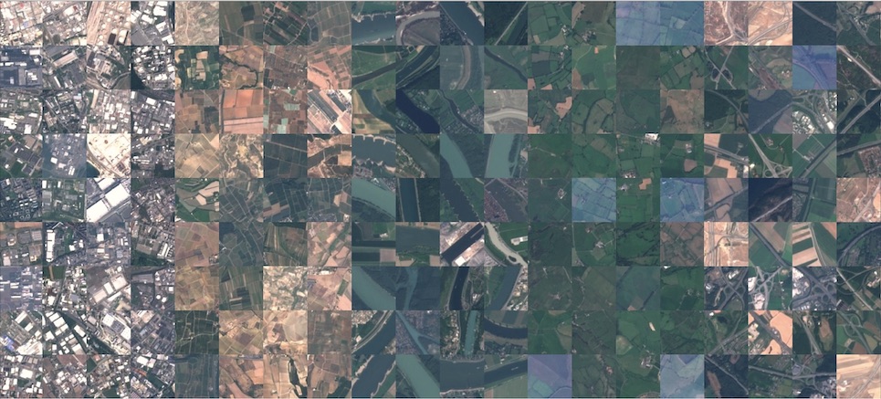
The EuroSAT dataset used in this tutorial consists of Sentinel-2 satellite images labeled with corresponding land use and cover categories. It provides a comprehensive representation of various land features. The dataset comprises 27,000 labeled and geo-referenced images, divided into 10 distinct classes. The multi-spectral version of the dataset includes all 13 Sentinel-2 bands, which retains the original value range of the Sentinel-2 bands, enabling access to a more comprehensive set of spectral information. This dataset has been published on the dedicated STAC endpoint.

Inputs

This application supports training the Convolutional Neural Network (CNN) model using either CPU or GPU to accelerate the process. It accepts the following input parameters:

Parameter	Type	Default Value	Description
stac_reference	`str`	`https://raw.githubusercontent.com/eoap/machine-learning-process/main/training/app-package/EUROSAT-Training-Dataset/catalog.json`	URL pointing to a STAC catalog. The model reads GeoParquet annotations from the collection's assets.
BATCH_SIZE	`int`	`2`	Number of batches
CLASSES	`int`	`10`	Number of land cover classes to classify.
DECAY	`float`	`0.1`	Decay value used in training.
EPOCHS`\|`int`	required	Number of epochs
EPSILON`\|`float`\|`1e-6`	epsilon value (Model's heyperparameter)
LEARNING_RATE`\|`float`\|`0.0001`	Initial learning rate for the optimizer.
LOSS	`str`	`categorical_crossentropy`	Loss function for training. Options: `binary_crossentropy`, `cosine_similarity`, `mean_absolute_error`, `mean_squared_logarithmic_error`, `squared_hinge`.
MEMENTUM	`float`	`0.95`	Momentum parameter used in optimizers
OPTIMIZER	`str`	`Adam`	Optimization algorithm. Options: `Adam`, `SGD`, `RMSprop`.
REGULARIZER	`str`	`None`	Regularization technique to avoid overfitting. Options: `l1l2`,`l1`, `l2`, `None`.
SAMPLES_PER_CLASS	`int`	`10`	Number of samples to use for training per class.

Outputs:

mlruns: Directory containing artifacts, metrics, and metadata for each training run, tracked and organized by MLflow.

How the training process is structured internally

The training pipeline for developing the training module encompasses four main components including:

Data Ingestion
Based Model Architecture
Training
Evaluation

The pipeline for this task is illustrated in the diagram below:

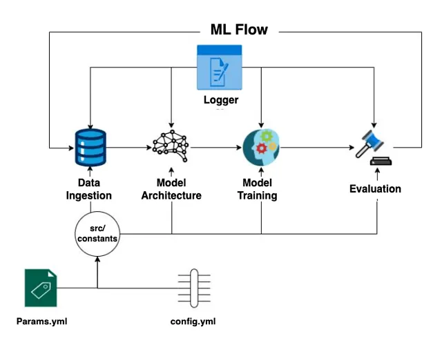
Data Ingestion

This component is designed to fetch data from a dedicated STAC endpoint containing a collection of STAC Items representing EuroSAT image chips. The user can query the collection using DuckDB on a GeoParquet file and split the resulting data into training, validation, and test datasets.

Based Model Architecture

In this component, the user will design a CNN composed of seven distinct layers. The model beginnings with an input layer, which accepts images of shape (13, 64, 64) or any other cubic image shapes (e.g. (3, 64, 64)). This is followed by four convolutional blocks, each of which consists of the following sequence:

A Conv2D layer with ReLU activation
A BatchNormalization layer
A 2D MaxPooling layer
A Dropout layer

Although each block contains multiple operations, they are collectively treated as four convolutional layers in the context of the model architecture.

After these convolutional blocks, the model includes a dense (fully connected) layer, typically used to transition from the convolutional feature extraction to classification. Finally, the output layer is a Dense layer with 10 units (corresponding to the number of output classes) and uses the softmax activation function to produce a probability distribution over the classes.

The user is required to select an appropriate loss function and optimizer from the available options. Once configured, the model is compiled and saved under output/prepare_based_model.

Training

This component is responsible for training the model for a specified number of epochs, as provided by the user through the application package inputs.

Evaluation

The user can evaluate the trained model, and MLflow will track the process for each run under a designated experiment. Once the MLflow service is deployed and running on port 5000, the UI can be accessed at http://localhost:5000.

MLflow tracks the following:

Evaluation metrics, including Accuracy, Precision, Recall, and the loss value
Trained machine learning model saved after each run
Additional artifacts, such as the Loss curve plot during training, and the Confusion matrix.

For developers

The folder structure is defined as: src/ tile_based_training / - components / - Containing all components such as data_ingestion.py, prepare_base_model.py, train_model.py , model_evaluation.py, inference.py. - config / - Containing all configuration needed for each component. - utils / - to define helper functions. - pipeline / - to define the order of executing for each component.